cs284a_hw2_webpage

webpage for cs284a

---

Project maintained by ZJUHSY Hosted on GitHub Pages — Theme by mattgraham

Project2: MeshEdit

Project Overview

In this project, we have explored the geometric modeling step by step and finally implemented the loop subdivision of mesh upsampling. Firstly, we build Bezier curves and Bezier surfaces according to the de Casteljau’s algorithm, and then we apply these methods to the actual graphics. Here, we come into contact with the Half-Edge Data Structure, which brings great convenience for us to deal with unit graphics through extensive definitions. We implemented normals and some structural transformations in the data structure, including flip and split, which are common components of Loop subdivision. Finally, we integrated them to complete the exploration of geometric modeling.

Part1: Bezier Curves with 1D de Casteljau Subdivision

1-1 Briefly explain de Casteljau’s algorithm and how you implemented it in order to evaluate Bezier curves.

Explanation:

The de Casteljau’s algorithm can calculate the points C(u), u∈[0,1] on the Bezier curve by a set of u values, we can calculate the coordinate sequence on the Bezier curve and draw the Bezier curve by it.

In the simplest case, We select a point C on the vector AB so that C divides the vector AB into u:1-u. Given the coordinates of points a and B and the value of u, we can calculate the coordinates of point C by C = A + (B - A) * u = (1 - u) * A + B * u.

The de Casteljau’s algorithm makes full use of this property. It uses the above method in each segment of a polyline to calculate the u:1-u segmentation points in the polyline, then connects each segmentation point to obtain a new polyline, and continues to use the segmentation method recursively on the new polyline until there is only one point left, the de Casteljau’s algorithm can ensure that the point must be on the Bezier Curve. Then, by changing the values of u, we can get the complete Bezier Curve of a polyline.

Implementation:

To realize the de Casteljau’s algorithm, we need to modify the function evaluateStep(). At the beginning of the function, we need to judge whether the number of input points is 1, which will be the termination condition of recursive call to the function. Then we use the LERP calculation method to calculate the segmentation points between each two points, store them in a vector, and then return the whole vector. When using the evaluateStep() function, we need to call it recursively, that is, the output result of the previous call is used as the input of the next call, until there is only one point left.

1-2 Take a look at the provided .bzc files and create your own Bezier curve with 6 control points of your choosing. Use this Bezier curve for your screenshots below.

1-3 Show screenshots of each step / level of the evaluation from the original control points down to the final evaluated point.

Because there are four original points, it takes three evaluations to get the final point.

Original point: First evaluation: Second evaluation: Third evaluation and get final point:

1-4 Show a screenshot of a slightly different Bezier curve by moving the original control points around and modifying the parameter t via mouse scrolling.

Part2: Bezier Surfaces with Separable 1D de Casteljau

How de Casteljau algorithm extends to Bezier surfaces?

Beizer Surface is similar to a high-dimensional version of Beizer curves. For each point, we define a (u,v) point, which u will produce a final beizer curve for one row of control points. Therefore, we will produce a list of control points for each row. And v will determine the final surface point along those moving curves.

Implementations

We first use lerps to caculate control points in each stage. And then we capsulate the evaluate1D function calling the evaluateStep for one step iteratively. Therefore, evaluate1D will produce a moving curve point for each row of control points. And finally function evaluate will call evaluate1D for each of its rows and produce the final surface point mentioned above. Picture 2-1 shows the final rendering output of teapot.bez.

Part3: Area-Weighted Vertex Normals

Implementation

We can use the normal method defined in the face class to calculate the normals for each face. Besides, we can use the formula to calculate the area of each face.

Hovwever, the most important part of this implementation is to traverse the faces (triangles) surrounding the vertice. To traverse adjacent face, we can use the half edge strcuture. Each step of the loop we calculate the weighted normals of the face where current half edge belongs to. And we can use h->twin->next->next to access the next surrounding face.

####Results Picture 3-1 is the result of our implementation after Phong shanding. We can see that the teopot is smoother compared to normal shading.

Part4: Edge Flip

4-1 Briefly explain how you implemented the edge flip operation and describe any interesting implementation / debugging tricks you have used.

Explanation of Implementation:

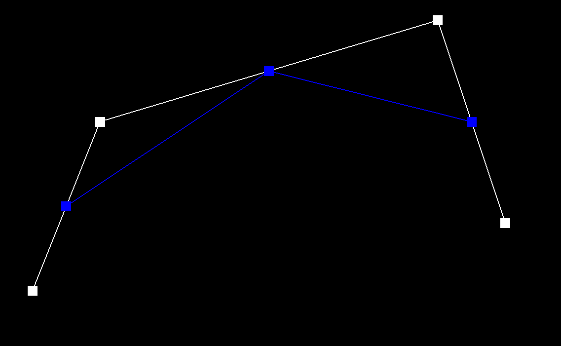
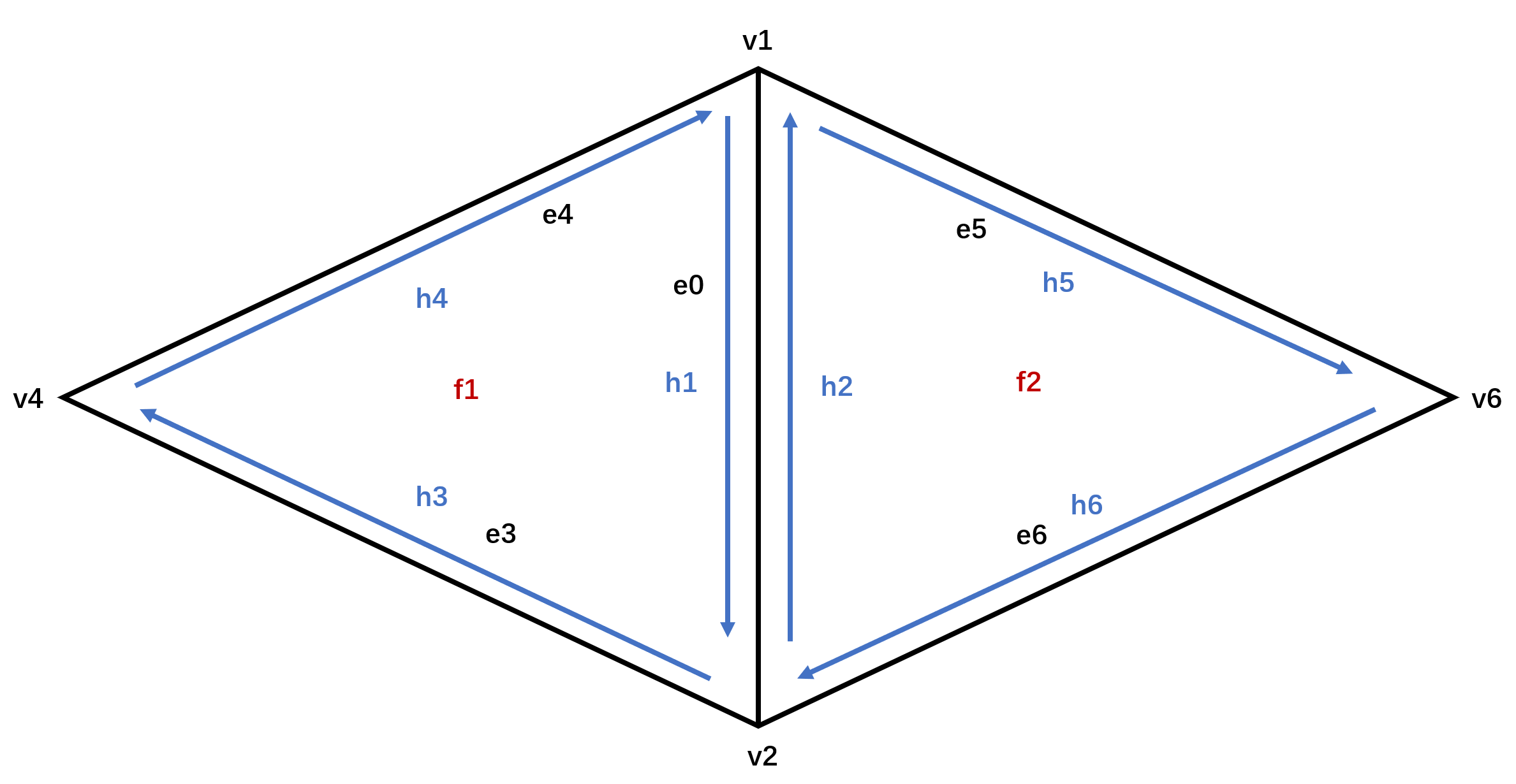
The original example is as follow, before starting coding, we marked out each Halfedge, Vertex, Edge and Face in the figure according to the provided data structure. In the process of code implementation, we first start from e0, traverse the whole quadrilateral, and define the variable name according to the name marked in the figure. The essence of edge flip operation is to eliminate one diagonal edge and then add edge to another diagonal. Before implementation, we also draw the expected result figure as a reference, and then modify it through the setNeighbors() function according to the Halfedges shown in the figure, and then modify other properties.

Debugging tricks:

The overall difficulty of this task is moderate, but the implementation requires a lot of processes, and it is not easy to debug after meeting errors. We need to complete it carefully and methodically.

It is necessary to determine the name of each variable before writing code, which can help us judge whether the traversal and modified topology is correct in real time. Secondly, in the process of writing code, we need to complete it in a certain order, either in the order of each structure type or in the order of all elements related to each Face. It should be noted that if we choose each structure type as the order, we’d better start with Halfedge, because halfedge is associated with each other, and other structure types are not necessarily associated with each other.

4-2 Show screenshots of the teapot before and after some edge flips.

Before edge flips:

After edge flips:

4-3 Write about your eventful debugging journey, if you have experienced one.

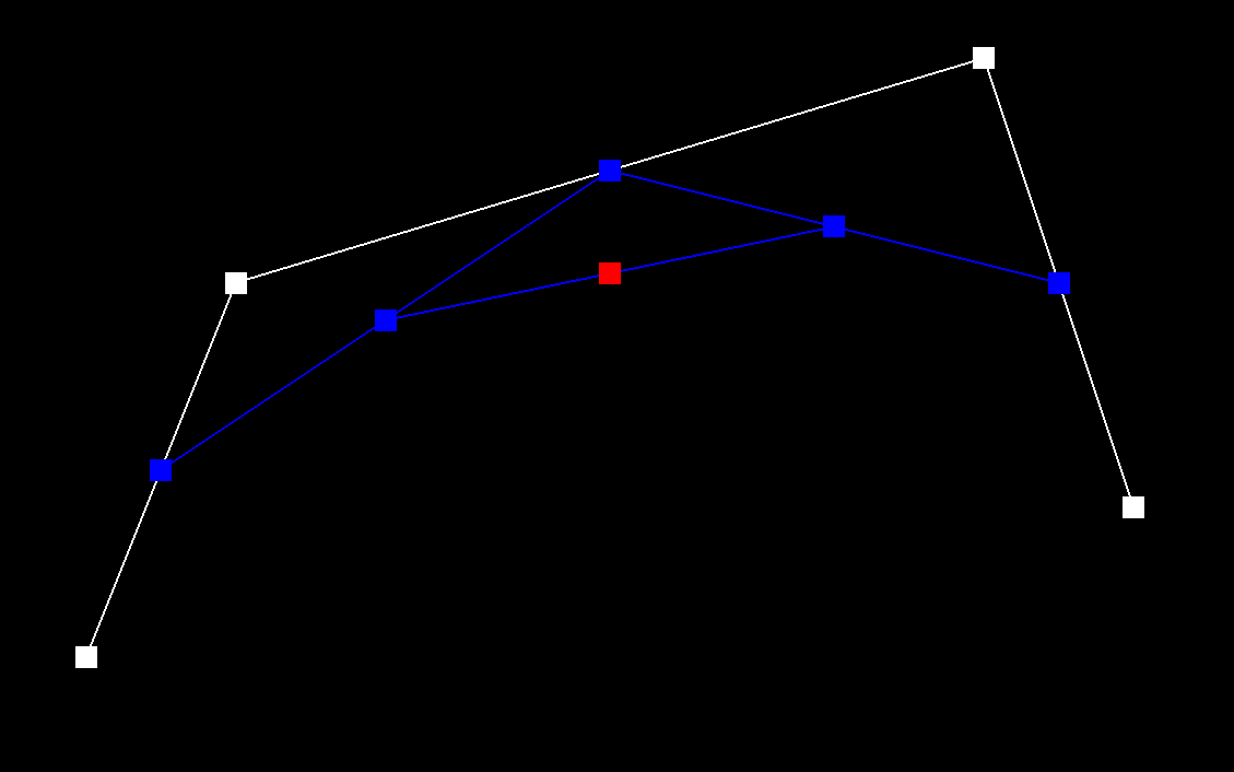
In our first attempt, we didn’t draw a clear image in advance as a reference, but wrote code according to intuition. In the result of flip, H1 and H2 were in the opposite direction, as shown in the figure below. In this case, ordinary flip can still succeed, but because the sequence closed loop is not formed inside the triangle, there will be a vacancy after multiple flips. As shown in the figure below. We tried to transform repeatedly in the figure and looked at each Halfedge direction to track the bug, then found the reason in the code logic, and finally modified it correctly. This is an unforgettable debugging experience which reminds us that when the brain can’t remember everything clearly, we should draw it down as a reference.

Part5: Edge Split

5-1 Briefly explain how you implemented the edge split operation and describe any interesting implementation / debugging tricks you have used.

Explanation of Implementation:

The principle of edge split is similar to that of edge flip, except that split does not eliminate the original diagonal, but adds a new connection between the middle point and the other two vertices on the basis of retaining the original diagonal. The operations needed to modify various parameters are basically the same as edge flip. The biggest difference in the implementation is that edge split adds a new intermediate point. Similarly, before starting coding, we marked out each Halfedge, Vertex, Edge and Face in the figure according to the provided data structure. In Part4, because the setNeighbors() function needs to input the twin of Halfedge, we also define the twin of border when traversing the initial structure. However, in Part5, since the number of variables increases significantly, we no longer define the twin of border, but directly enter Halfedge->twin in setNeighbor(), which can simplify the code. The rest of the implementation methods are similar to those in part 4. First traverse each structure in the original figure, then initialize new vertex and face, and finally update all variables.

Debugging tricks:

The trick of this part is similar with Part4. It is necessary to determine the name of each variable before writing code, which can help us judge whether the traversal and modified topology is correct in real time. Secondly, in the process of writing code, we need to complete it in a certain order, either in the order of each structure type or in the order of all elements related to each Face. It should be noted that if we choose each structure type as the order, we’d better start with Halfedge, because halfedge is associated with each other, and other structure types are not necessarily associated with each other.

5-2 Show screenshots of a mesh before and after some edge splits.

Before edge splits:

After edge splits:

5-3 Show screenshots of a mesh before and after a combination of both edge splits and edge flips.

Original:

After edge flip:

After the combination of both edge splits and edge flips:

5-4 Write about your eventful debugging journey, if you have experienced one.

After obtaining the experience of Part4, we carefully drew the reference figure, clarified the logic before writing the code, and achieved BugFree in this part!!!

Part6: Loop Subdivision for Mesh Upsampling

Implementation

We follow the instructions listed on the rubrics. In the first part of our implementation, we first pre-calculate and store the updated coordinates for both new vertices and old vertices using the loop subdivision rule. To be more specific, we store the updated positions in VertexIter->newPosition for old vertex, EdgeIter->newPosition for new points.

In the next step, we split and flip every edge in the mesh. To avoid splitting new edge, we only split edges that are connected by two old vertices. To flip each edge after splitting, we flip only new edges that are connected by a old vertice and a new vertice. The details are tricky here. If we label the two edges that are splitted by the middle points as new edges, it will be difficult to determine which edge to flip. Because we will end up flipping those edges because they are connected by a new vertex and an old vertex, which will produce infinite loop.

Instead, we label those aforementioned two splitted edges as old edge by the data strcuture. And we only split those edges that are connected by two old vertex and flip edges that are new and connected by an old vertex and a new vertex. This will resolve the problem mentioned above. (We use EdgeIter->isNew and VertexIter->newPosition to label whether a point and an edge is new or old.)

Sharp Corners And Edges

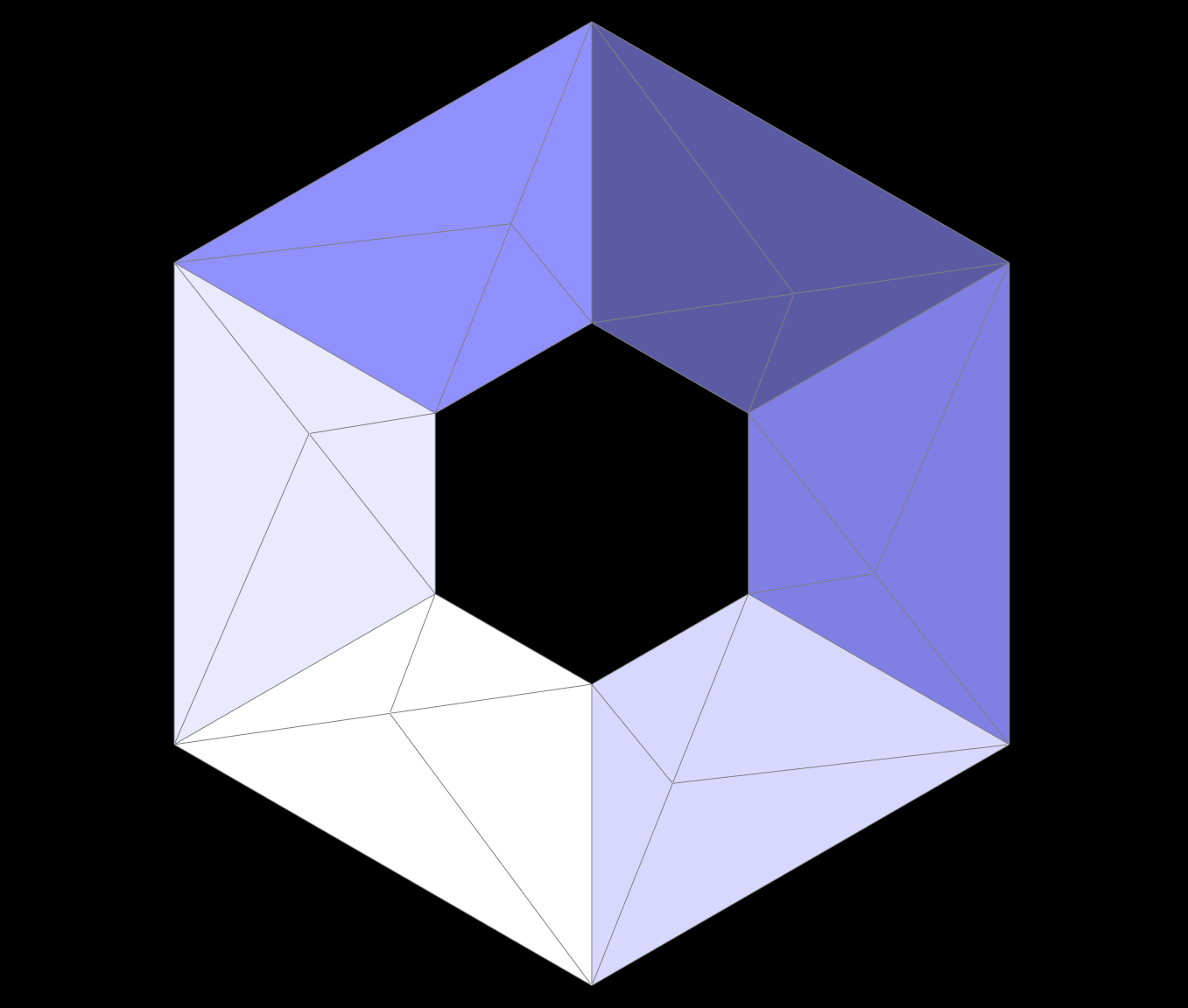
During the experiment, we found that the graphic density of some sharp corners and sharp edges will increase after edge split, resulting in uneven distribution of the whole image at the original corner, as shown in the figure below.

Corner before split:

Corner after split:

We think this may be related to the corresponding degree of angle of the corner in 3D space. If the corner is spliced by the three right angles shown in the above figure, the density will be uneven after multiple splits. However, if we splice the corner into three 60 degree angles through flip and split, as shown in the figure below, the image will still maintain uniform density after multiple split.

Corner before split:

Corner after split:

In order to verify our assumption, we choose another corner spliced at an angle of 60 degrees, and we also get a uniform graphic distribution after split.

Corner before split:

Corner after split:

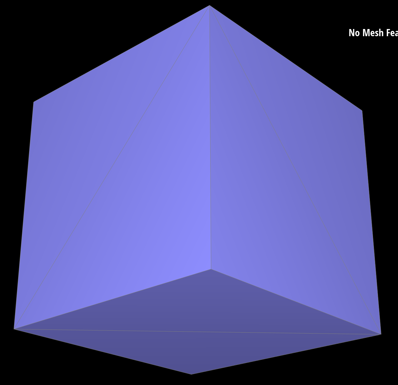
Asymetric Problems

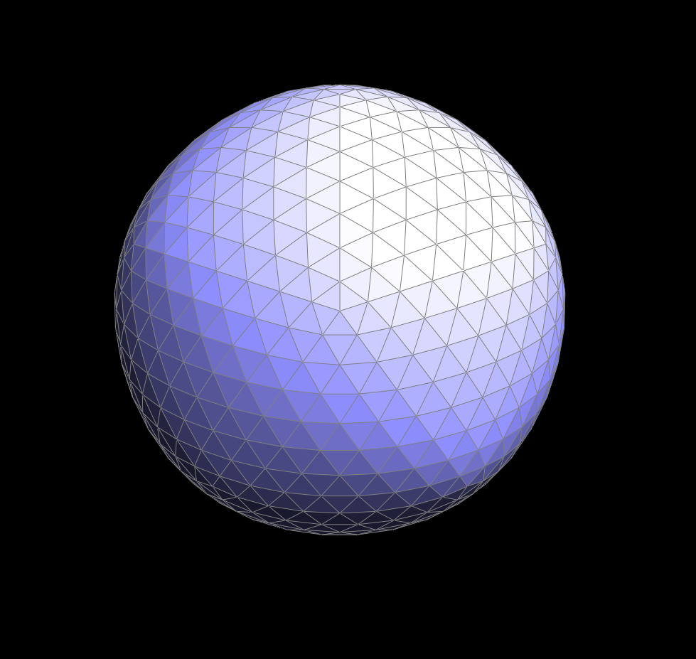
As illustrated on the figures, the cube become asymetric as loop subdivision continues (picture 6-3-1, 6-3-2, 6-3-3). This can be explained that the original square is not symmetric. And there are two ways to make is symmetric: 1. split 2. flip

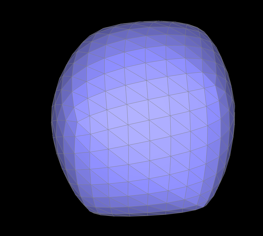
We can first see the power of splitting edges. We split each diagonals in the square to make every face symmetric. We can see from picture below the magic of pre-splitting the diagonals. Though the shape is symmetric, the texture is not.

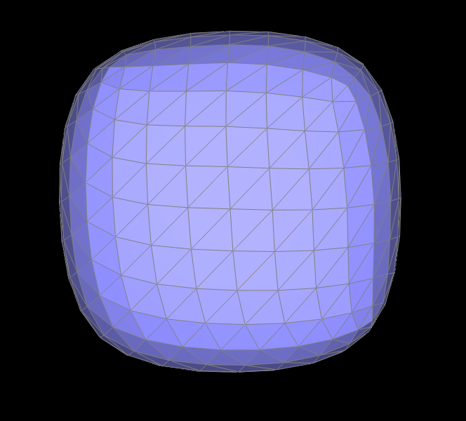
Therefore, we can use flip to make the whole cube symmetric, both shape and texture. The procedure (including the original cube after flipping the diagonals to mkae it symmetric is shown below).

Webpage Link

Our web page is deployed at website.